I Have Met the Efficient Market, and It Is Us
There’s a famous mathematical puzzle that goes something like this: on an island, there live 200 supremely rational, law-abiding, non-suicidal people, some of whom have brown eyes and some of whom have blue eyes. They are bound by a sacred rule: they must not learn the color of their own eyes. If they do, then they must kill themselves by nightfall. One day, a green-eyed fairy descends from the heavens and proclaims, “I see at least one person who has blue eyes.” What happens?
I won’t dissect this puzzle in detail, as others have already done so. The crux of the solution (spoiler alert!) lies in understanding that even if everybody knows a certain fact (everybody can see blue-eyed people around them), the public statement of that fact can still add information to the public knowledge—sometimes with drastic consequences!
I immediately thought of this puzzle after reading Josh Barro’s alleged debunking of the efficient market hypothesis. The efficient market hypothesis says, roughly, that the price of a security incorporates all publicly known information. Now, this isn’t really a “hypothesis” in the scientific sense of the word, since it’s not making a concrete, testable prediction, but that never seems to stop people from trying to refute it.
Barro’s argument goes as follows. On Thanksgiving, he wrote an article about falling prices of taxi medallions. This wasn’t some big investigative scoop—the few people who pay attention to taxi medallion prices already knew that prices were falling. Barro merely put that information in a prominent place, the front page of the New York Times the following morning. When the stock market opened on Friday, the stock of Medallion Financial, which invests in loans secured by taxi medallions, was down 6%.
Aha! Gotcha, efficient market hypothesis! Despite no new information being released to the public, and nothing else substantial changing in the taxi medallion situation between Wednesday’s close and Friday’s open, Josh Barro single-handedly tanked Medallion’s stock. But wait—is it really true that no new information became available? Even if everybody already knew the information in Josh’s article, the fact that it appeared on the front page of the New York Times brought the situation to a head. Now, everybody knows that everybody knows. More to the point, if I’m a canny trader and I read Josh’s article in the morning paper, I picture hordes of mindless retail-investing zombies shambling over each other in an attempt to sell off their shares of Medallion. What this means is that there’s a great buying opportunity somewhere well below the current price, so certainly I shouldn’t be trying to buy anywhere near where the stock was on Wednesday’s close. And if I hold Medallion, I need to sell—fast!—hoping to catch the one buyer who was in too much of a hurry to read the paper that morning.
“Buh-buh-but,” you may object, “that has nothing to do with the fundamentals of the company! It’s based on a bunch of people behaving irrationally!” Well, tough cookies! Nobody said anything about people behaving rationally, or that the price would clearly reflect the company’s fundamentals. The market is doing exactly what the efficient market hypothesis says it does: it’s incorporating new public information instantly. It just happens that the relevant information is not the information contained in the article, but rather the effect that information will have on the buyers and sellers in the market.
Here’s the thing. Let’s say you think you’ve found some inefficiency in the market. Do you (a) exploit it to make lots of money, or (b) decide you can’t be bothered and maybe write an article crowing about how you’ve debunked the efficient market hypothesis? If, like most financial pundits, you choose option (b), then you haven’t really proved anything, since at a bare minimum, you need to show you can actually buy low and sell high based on whatever public information you think hasn’t been incorporated into the price. And if you choose option (a), well, you’re using your human and technological capital in exchange for a profitable trade. Markets are collections of human beings and machines who turn (typically) public knowledge into profitable trades. Seeing a profitable trade without any secret information doesn’t disprove the efficient market hypothesis: making that trade is what makes the market efficient.
If this all sounds like a load of sophistry, it is, but there’s nothing wrong with that. As I said before, the efficient market hypothesis shouldn’t be taken as a statement of scientific fact, but rather as a lens through which we can try to understand how markets work. I would argue that, contrary to the claim that people exploiting public information for profit disproves the efficient market hypothesis, the efficiency of markets is what makes trading financial products even possible. If you had to know everything there is to know about a financial product in order to be able to trade it without worrying that it’s horribly mispriced, then nobody would ever trade anything. It’s the confidence that, to first approximation, everything is priced correctly that allows traders to actually do what they do.
Type Checking the Inequality Debate
Facts are meaningless. You can use facts to prove anything that’s even remotely true!
—Homer J. Simpson
I’ve already thrown in my two cents on the central theory in Thomas Piketty’s Capital in the 21st Century. But I think (again, not having actually read the book) that the legacy of Capital will not be its theory or its policy prescriptions, but how it has shaped the debate on inequality. In the past, even as recently as the Occupy Wall Street movement of a few years ago, ideology took center stage. Piketty’s rise to stardom has put the spotlight on data.
On the one hand, this is a terrific development. Ideological debates are intractable, while data can, in principle, be viewed and discussed in an objective manner. But data analysis has its own pitfalls, and if we’re not careful, our own ideological biases might seep into the data we choose to study and present. What we need is an expressive but strict framework with which to view data: expressive meaning we can uncover the truth hiding in the data, and strict meaning we won’t erroneously use the data to say something false. What we need, in other words, is dependent type theory.
One common theme in data cited by those on the “left” of the inequality debate is the rising gap between the top 1% (the choice of 1% being an unfortunate vestige of Occupy that should be snuffed out ASAP) and everybody else. Consider the chart below from Christopher Ingraham’s Wonkblog article, More reasons why the U.S. is the best place to be rich, which shows the income share of the top 1% rising dramatically in the United States from 1981 to 2012. Can you spot the type error?
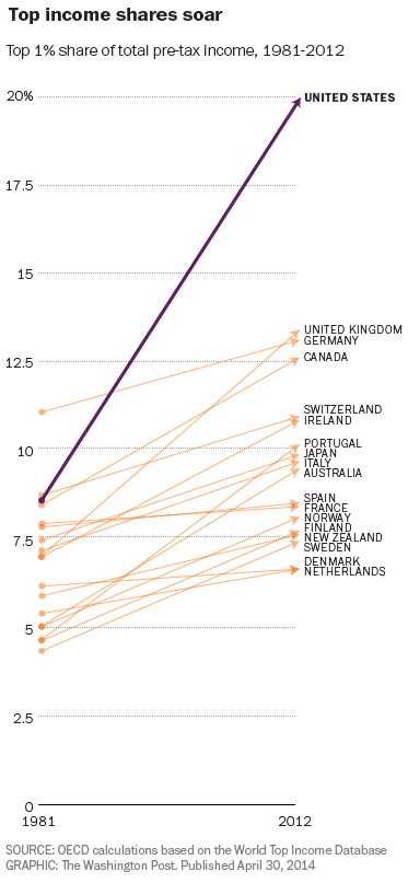
Did you find it? No? Well, let’s consider the dependent variable here. In order for a chart to make sense, the type of the dependent variable needs to be constant: it can’t depend itself depend on the independent variable (in this case, time). This is, for instance, why we need to choose a particular year to discount to in charts of dollars vs time: in general, the type of money depends on time!
The problem in this chart is a bit more subtle: the people who comprise the top 1% change over time. This is not merely a technical consideration. You can easily imagine a society with a high level of mobility in which people routinely rotate in and out of the top 1%. In such a society, is a chart like the one above really indicative of any problem? While we aren’t quite at that level of mobility, Thomas A. Hirschl and Mark R. Rank found that 12% of Americans are in the top 1% for at least one year, and 73% are in the top 20%. This dynamic view of income distribution is made completely invisible by Ingraham’s chart.
So, Ingraham’s chart fails my internal type checker, and in my opinion, such charts should not exist. Don’t get me wrong: I think inequality is a huge problem (albeit much more so on the global level than domestically). But it serves no one to make misleading presentations of data. Often the desire to be righteous blinds us to the virtues of being right. Until we have a system that can automatically type check our data analyses and presentations, we need to be extra vigilant ourselves to make sure that what we’re doing with data actually makes sense. Friends don’t let friends make type errors. So be a mensch: type check your friends, not just your enemies.
Why Dependently Typed Programming Will (One Day) Rock Your World
You can #timestamp it, folks. I’ve seen the future, and it’s dependently typed. We won’t merely teach the homeless to code. Rather, me and you and everyone we know will have a whole new framework in which to think, learn, and interact with the world. When the day comes to start running software on our brains, we’ll only need to upload one program: a type checker.
I know what you’re thinking: he’s totally lost it. I was like you once. My eyes were closed to the endless possibilities of dependent types. But don’t worry, I’m here to awaken you.
All right, what you’re actually thinking, assuming you’re still reading this, is “what the heck are dependent types, and why is this man getting so unreasonably worked up about them?” I will try to contain my mælstrom of emotion long enough to answer. I’m going to be incredibly vague and probably wrong. Deal with it.
Programming languages can be roughly divided into two classes: imperative languages and functional languages. In an imperative language, you tell the computer what sequence of steps it should take to solve a given problem. In a functional language, you describe the problem to the computer, and it solves it for you. (I did say this was going to be incredibly vague and probably wrong!) Now, you might think that the second way is the way to go because the first way requires you to do the hard work of figuring out how to solve the problem. Let’s have the computer do that, right?
The problem is that like your in-laws, computers are hard to talk to. The languages they speak tend to have limited expressivity. Describing how to solve a problem step-by-step doesn’t require expressing very much (do this, then do that, carry the 2, mumble grumble), the questions we want the computer to help us answer, if they’re at all interesting, tend to be much grander in scope: we might be trying to answer questions that are out in the real world. As scientists (and even as regular people), we greatly simplify the real world with models, but even describing your model to a computer can be hard because everything needs to be made very precise. And while it is unquestionably a Good Thing™ to make your models precise, doing so in the context of a computer language can be a tortuous process: it’s easy to get lost in the process of translation and not realize when we’ve made a conceptual error.
This is the fundamental flaw with most programming languages, particularly the functional kind. The process of honing a model should be edifying, but instead we are forced to translate the beautiful poetry that pours out of our brains into a grunty computer tongue. Yes, many people have gotten very good at this process! But I think they are good at it in spite of the tools they’re using. What we really need is a programming language with a word for X, where X is a concept relevant to the problem at hand. We need a programming language that will chide us not just when we’ve made a grammatical error but also when we’ve said something whose meaning is not quite right, like “vaccines cause autism.” In other words, we want the computer to understand not just our syntax, but our semantics.
Now I need to tell you about types. In procedural languages, we (typically) have the notion of a data type, which is just a label we attach to pieces of data that say what type of data they are. So we might attach the label int (short for integer) to the data 8, or the label string to the data "Hello, world!". If you’re lucky, your procedural language will care enough about types to tell you when you’ve done something silly with them: it’ll OK adding 8 and 4, but not adding 8 and "Hello, world!" But it will also OK dividing 8 by 0. Note that I am talking here about compile-time behavior. When you actually run your program that divides 8 by 0, the universe will implode. (As we all know, that’s what happens when you try to divide by zero.)
If you’re a smart cookie, you might try to prevent the cessation of existence itself by writing your own dividing function that checks first to see if you’re trying to divide by zero. Here’s some pseudo-code:
float myDivide(float a, float b) {
	if (b == 0)
		return ???;
	else
		return a / b;
}
The function, myDivide, takes two floating-point numbers a and b, and returns their quotient, which is another floating point number. We want to check first that b isn’t zero before dividing them. The problem here is that we don’t know what the function should output if b does happen to be zero. The function has to output some floating point number! Now, if we’re lazy, we might just pick some number to output in this case, like 0. After all, we’re just trying to prevent the universe imploding here: we don’t actually plan on dividing by zero and then trying to use the number we get out of it! The problem, of course, is that we might not realize we’re trying to divide by zero. If we are, then something’s definitely wrong, and we want to know about it!
At the heart of the matter is the fact that the mathematical operation we’re trying to implement, division, doesn’t just take two numbers a and b and output a third. We have to be precise, remember? It takes a number a and a non-zero number b, and outputs a third number. So what we can do is create a new type, nonzerofloat, to represent any floating point number that isn’t 0. Then, we can just define our function as follows:
float myDivide(float a, nonzerofloat b) {
	return a / nzfloattofloat(b);
}
Here, nzfloattofloat is an auxiliary function that takes as input a nonzerofloat and outputs that number as a float. Now, if we try to do myDivide(8, 0), the compiler will yell at us because 0 doesn’t have type nonzerofloat. What we’ve done here is to increase the expressiveness of the type system: an error that would’ve imploded the universe at runtime is now caught by the type checker.
This is solution 1 (of an eventual 3) to the divides-by-zero problem. And to be honest, it stinks. Why? Because if your program is doing some highfalutin computations, you’re not just going to be dividing explicit numbers. You’re going to need to divide the result of one computation by the result of another computation. And how do you know the result of that other computation isn’t zero? The type checker certainly doesn’t. And you can’t even do something like
if (bar != 0) baz = myDivide(foo, bar);
because the type checker can only check types; it doesn’t have access to the computation bar != 0 because that computation won’t be performed until the program is run. We need to do better.
Functional programming languages up the game by using types to describe not just data but functions as well. So the function
int plusOne(int a) {
	return a + 1;
}
which takes an int and outputs another int will itself have the type int -> int.
Why is this useful? One reason is that it allows us, in a fancy-pants language like Haskell, to instantiate our functions inside various computational contexts, or monads as they are called to scare you. For example, one computational context is lists. A list [2, 3, 4] of integers will have a type [int] or list int. We can also apply the list functor to our function plusOne. So while plusOne had type int -> int, the function [plusOne] has type [int] -> [int]. And it does exactly what you think it should: [plusOne]([2, 3, 4]) = [3, 4, 5].
But the functoriality isn’t why monads are interesting. I called lists a computational context, but come on, you can do that with a for loop. The interesting part of lists is that they can represent non-deterministic computations. For instance, we might want to define a “function” that takes an integer and returns a proper divisor of that integer. Now, this isn’t really a function between integers, because a number can have many divisors. But we can define a function divisor of type int -> [int] that returns the list of all divisors. Now I might want to chain together a number of such “non-deterministic functions” into a larger non-deterministic computation. Let’s say I want to pick a digit of a divisor of a number. I have the divisor function that sends a number to its list of divisors, and then the digit function that sends a number to its list of digits, both of type int -> [int]. Now, I can’t compose these two functions directly, because the output of divisor is of type [int] while the input of digit is of type int. But if I do what I did with plusOne above, I can feed the output of divisor into the function [digit]: [int] -> [[int]] that takes a list of integers and returns a list of lists of digits. The last step is to concatenate all these lists of digits to be left with a single list.
Whew. Let’s go back to division. One of the simplest Monads is the Maybe monad. You can think of it as a list with either 0 or 1 element: something of type Maybe Int is either a 1-element list like [4] or the empty list []. Whereas the list monad allowed us to describe general non-deterministic computations, the Maybe monad allows us to describe computations either have a definite answer or no answer. Like dividing by zero!
(Maybe float) myDivide2(float a, float b) {
	if (b == 0)
		return [];
	else
		return [a / b];
}
This looks a lot like our original attempt, but now we have a separate symbol to return in the case of division by zero. What’s more, functoriality lets us chain this Maybe-function together with ordinary functions, and our fancy concatenation procedure (called “binding”) lets us chain this Maybe-function with other Maybe-functions.
So this is our second solution. It’s not bad, I guess. Why am I not enthused? Because at the end of whatever grand computation we do, we’ll maybe have an answer. We still won’t know until we actually run the program! While this is undoubtedly more graceful than allowing the universe to implode, it still leaves a sour taste in my mouth. All we’ve really done is built a fancy machine for propagating the fact that we screwed up throughout the rest of our program. We might as well just interrupt our program on dividing by zero, which is how procedural languages handle things.
In a procedural language, the type checker just knows about data types. Any sort of error handling or more enlightened analysis of what’s going on needs to be inserted in a very ad hoc manner. In a functional language, the type checker knows about function types. This lets Haskell programmers do very fancy things to protect the universe from implosion, but not only can this become very hard to understand once we start putting monads in monads, it also ultimately doesn’t really help us: we still need to run the program to observe that the computation fails somewhere and then figure out what happened.
The problem with all of these programming languages is that they don’t get us. They don’t get what we’re trying to do. We never actually want to divide by zero. If we want to divide by something, we have a reason to believe that it’s nonzero. What we need to do is to make our beautiful brain poetry, our reason to believe that what we’re dividing by is nonzero, precise. We need a proof. Without further ado, here’s our final, most glorious division function:
float myDivide3(float a, float b, proof(b != 0) p) {
	return a / b;
}
What’s going on here? Our function takes three arguments now: our old friends a and b, together with a new guy, p. This new guy is a proof that b is nonzero, and its type depends on the value of b. This means that whenever I call this function, I need to provide together with a and b a proof that b isn’t zero. This may seem cumbersome, but like eating our vegetables, it’s good for us: it makes us clarify why we think we can divide by b at all. If you can’t do that, you have no business dividing!
The interior of this function is a lie, but a suggestive one. I wanted to make it clear that this function will always return a / b. Always. No maybes, no world imploding; we’re going to get a real, honest floating point number out of this function every time. In reality, the interior of our function will be some implementation of a division algorithm, which will use the fact that b != 0 to show that the algorithm terminates.
Allowing dependent types is the final piece of the puzzle. In a dependently typed programming language, a program isn’t just a program, it’s a computer-verified proof that your program will terminate. The language of dependent type theory allows us to express all of our beautiful thoughts about why the pieces of our model fit together the way we think they do. We might, in the process, discover that things don’t actually fit together right: the type checker will growl at us if they don’t. This can be tough if you’re just learning a language. But look at the upside: it won’t let us write bad code!
So why do I think that dependently typed programming is insanely great? It has to do with how we reason, and how we can learn to reason better. I’ve observed, teaching mathematics, that many of the fundamental errors students make are type errors. For instance, a beginning linear algebra student might try to find a subspace of a single vector. (Qiaochu Yuan has a very nice post expounding on these sorts of errors.) It’s tempting, as a teacher, to ignore milder forms of such errors (like mixing up subspaces and bases of subspaces) when students can churn out answers that are at least identifiably correct. But type errors are at the very least a strong indication that there’s some conceptual misunderstanding. I’ve often felt that mathematics education could be greatly improved by implementing stronger typing in our teaching, making clear what sorts of operations can be performed on what sorts of objects.
Dependent type theory takes this idea and runs with it. Type errors are not just red flags: in a sufficiently well-specified theory, all errors are type errors. Of course, I’m excluding routine mistakes like arithmetic errors, but those are the least important kind now that we have computers to do routine calculations for us. Rather, reasoning within the type theory of mathematics helps prevent us from making conceptual errors.
If teaching dependent type theory to schoolchildren seems like a bit of a stretch, it is. But the beautiful thing about dependent type theory is that it is expressive enough to express much simpler languages. One such language currently under development is AML, a modeling language for actuaries. By the end of this brief overview of AML, I was ready to jump up and down on the table. Why? Because money is a dependent type! It depends on time! It doesn’t make sense to add, compare, or otherwise mix two different sources of money unless they’re discounted to the same time. This is an error that’s easy to make when reasoning about money if you’re not careful. But in AML, it’s a type error: you just can’t do it!
After reading that, I was ready to turn everything into a type error. Make a chart with misleading axes? Type error! Use massively bloated animated GIFs instead of HTML5 video? Type error, my friend! What a wonderfully refreshing view of the world. Since deciding to leave the friendly confines of academia and search for a real job, I’ve tried to find a programming language to call my own. Each one just didn’t feel quite right until I hit upon Idris, a dependently typed language with a Haskell-like syntax. Finally, here was a language that could think as I do. Idris, you get me. And while Idris is still in its early stages, I don’t think the day is too far off when we’ll be using Idris, or a language like it, or a language created with it, to do mathematics and science and statistics and learning and living and loving. And that day will be awesome.
The Capital Asset Pricing Model Is Not a Pricing Model
The Capital Asset Pricing Model (CAPM), which I discussed briefly in a previous post, says that the expected excess return of an asset is proportional to its on the excess return of the market portfolio, or more precisely,
One catchy way people tend to remember this is that the idiosyncratic volatility of a security doesn’t matter, only its market beta. But this is a vacuous statement: the idiosyncratic volatility is by definition a mean-zero quantity, so when we take expectations, it vanishes! In fact, the CAPM says nothing about the idiosyncratic volatility; rather, it says that the idiosyncratic mean is zero. Moreover, our catchy slogan directly contradicts one of the things we learn early on in our asset pricing careers, which is that, given that investors have some level of risk-aversion, increasing volatility should lower prices.
The confusion here comes from the fact that the CAPM, in the way it is usually stated, is not a pricing model: it’s a model of expected returns. And expected returns by themselves don’t really tell you anything about what prices should be: you need some absolute information like future dividends to anchor expectations to an absolute price. Indeed, price, as I explained in my very first post, is equal to the expected discounted payoff, that is,
Notice that the price cancels once we write the payoff in terms of the return, so we can’t really use information about returns alone to say anything about price.
So what does the CAPM say about prices? A lot, it turns out. This is because the condition is equivalent to saying that the market portfolio is mean-variance efficient; in particular, it is the tangency portfolio. The weights of the market portfolio are given by market capitalization, while the weights of the tangency portfolio are given by , where is the covariance matrix of all assets and is the vector of means. (This formulation only makes sense if the covariance matrix is nonsingular, but that’s not so important.) So the CAPM, in this form, explicitly relates the market capitalization of stocks to their means and covariances. In particular, if we add a completely idiosyncratic volatility to a single asset, this will reduce its weight in the tangency portfolio (which is just its market capitalization), and hence reduce its price.
Given that the CAPM entirely determines prices in terms of means and covariances, why did I claim that the CAPM is not a pricing model? Because the “true” means, and especially the “true” covariances, of assets are impossible to determine from data. The beta of a stock is a reasonably stable quantity, so the CAPM works pretty well to model returns, but its price implications, while quite elegant, are not really visible in the real world.
The Perils of Growth
Thomas Piketty’s new book, Capital in the 21st Century, has created a lot of buzz in the economics blogosphere. Having not actually read the book, I’d still like to throw in my two cents on the problem with (what I understand as) its underlying thesis. The 20th century, according to Piketty, was anomalous in its low level of inequality because the rate of growth of the economy was greater than the rate of return on capital . In the past, and increasingly so in the present day, , in which case the holders of capital become increasingly rich compared to the rest of the populace.
The central issue I see with this thesis is neglecting the role of consumption, and the decreasing marginal utility thereof. It’s hard to deny that the West in the 20th century saw both a great diminishment in wealth inequality and a great increase in general well-being, but we shouldn’t leap to the conclusion that the one caused the other. Not all growth is created equal, and we need to separate growth that improves well-being from growth that simply increases consumption and even worse, tends to shifts the utility curve to the right so that more consumption is required.
On the one hand, we eliminated horrific diseases like polio and smallpox and introduced enormously beneficial technologies like computers and the Internet. The greatness of these advancements lie in their increasing marginal utility with small marginal costs: the more people get vaccinated against deadly diseases and the more people use information technology, the better and cheaper these things become.
On the other hand, two of the worst trends of the 20th century were the increase in the prices of housing and transportation, the two categories which currently lead consumer expenditures. I’m sure it was great to be the first person in town with a car or the first family on its block to have a big house with a big yard. Cars are fun to drive, and a big part of the early thrill must’ve been beating out the plebes traveling by foot or by horse, and similarly for big houses. But today, driving a car is not only not fun (who enjoys being stuck in traffic?), but is now essentially a requirement to live and work in many parts of the US. Yes, it’s true that 20th century growth transformed the automobile from a luxury item into a necessity. And that’s bad! Before this wonderful “growth,” the average American didn’t need to spend a huge percentage of their income on transportation. And similarly for housing: now that many places have written single-family dwellings with plenty of yard and plenty of parking into law, people have little choice but to spend a hefty chunk of income on these things.
Inequality shouldn’t just be about absolute wealth numbers. It should be about how many people can actually make a living. And because of much of that 20th-century growth, we’ve vastly increased the requirements for making a living. Imagine if instead of the automobilized sprawl we created, we had built efficient, walkable cities with excellent transit. Then most of the money people now put towards paying for housing and transportation could instead be saved and invested. And investing today is easier than ever! If everybody shares in capital, we shouldn’t be concerned by a high rate of capital returns. But instead, we’ve forced people into serfdom to pay for “necessities” like cars and homes.
I’m not a luddite, nor am I necessarily anti-materialist. But I’m frankly alarmed by what has, through a combination of legislative fiat and societal pressure, become the minimum standard of living. A lot more people could make ends meet if we didn’t place the ends so far apart in the first place! There’s no reason why, for instance, a single person shouldn’t be able to live in a small studio apartment in a city for a couple hundred dollars per month within easy walking or biking distance of their job. But this is quite frankly impossible: anywhere with cheap enough housing will probably not be walkable or bikeable, because walkable and bikeable places are in limited supply and high demand.
Instead of the power of growth, let’s focus on the power of thrift. The 20th century was an amazing time for thrift! Entire industries are now obsolete due to the rapid progress of technology (though some, like academia, have yet to admit it). Globalization has made basic necessities like food, clothing, and furniture incredibly cheap. Could a person at the dawn of the 20th century even imagine how much of that stuff we simply throw out because we have such an embarrassing oversupply? Surely we must live in paradise! But our problems lie in our built environment. We’ve given up control of that to the bureaucrats, and the result is predictably miserable. Thrift is nowhere to be seen, but neither is quality. The appetite for bigger homes, wider streets, MOAR PARKING grew and grew over the course of the 20th century, and we are hardly better off for it. Before we become alarmed at the impending infrastructure budget shortfall, we should take a step back. Growth is not always good. Sometimes the answer is not more, but less.
Why Do People Trade?
There’s been a big brouhaha lately over the new Michael Lewis book, Flash Boys, which paints a picture of nefarious high-frequency traders swindling honest investors out of precious pennies every time they trade. I don’t feel I have much to contribute to the is-HFT-good-or-bad debate because I know very little about the actual mechanics of trading, which are necessary to understand what’s actually going on. Rather, I want to tackle a more fundamental misconception at the center of many people’s arguments, namely, the role that trading plays in the markets.
As I’ve mentioned several times before, you can’t go too wrong as an individual simply putting your money in a Vanguard total stock market index fund. Now, putting money in such a fund itself requires an act of trading, even if you’re buying into a mutual fund instead of an ETF: Vanguard needs to purchase more shares of stock to cover your investment. But once your money’s in there, no more trading needs to take place. There’s no need to “rebalance” a value-weighted portfolio of stocks, as the weighting of each stock is proportional to its price.
Even more complicated investment propositions should involve surprisingly little trading, in principle. One common (though possibly misguided) investment trope is that one should keep a constant ratio of stocks to bonds, say 60–40. If the value of your stocks go up relative to your bonds, you should “rebalance” by selling stocks and buying bonds. But now imagine that everybody is taking this advice. If stocks go up relative to bonds, then everybody is going to want to sell stocks and buy bonds. But that means nobody wants to buy stocks and sell bonds! So the price of stocks will have to drop, and the price of bonds will have to rise until the market clears, which happens, you guessed it, when everybody’s back to 60–40. So in fact, no trading ever takes place!
This story (which I should attribute, like most of my finance knowledge, to John Cochrane) highlights the fundamental misconception many people have about markets, that trading drives price changes. When the market goes up, the finance media explains it as people buying, and when the market goes down, it’s people selling. But this is transparently absurd: every transaction involves one buyer and one seller! No matter how the market does, the amount of stock bought is equal to the amount of stock sold. Indeed, there’s no reason whatsoever that price changes need to involve trading whatsoever. In a truly efficient market, if information comes in that affects the price of a stock, everybody should immediately update their quote values. If you learn that a stock that was trading at $20 is suddenly worth $30, you’re not going to find somebody who’s going to sell it to you at $21, even if they would have a second ago.
Let’s bring in some empirical evidence. A 2004 paper by Brandt and Kavajecz analyzes what drives movement in US treasury yields. First, they cite previous research that the largest changes happen immediately following scheduled macroeconomic announcements. Notably, these changes happen instantly, without any trading. This makes sense: everybody knows these announcements are going to happen in advance, so nobody’s going to leave stale quotes around to get sniped once the announcement is made. After the announcement, market participants can enter new quotes at a new price level.
Brandt and Kavajecz want to explain what causes changes in prices at other times. The mechanism they propose is called price discovery. The idea is based on the existence of information traders: people who have private information relevant to the market and trade based on this information. Information traders have a reason to trade: they know something you don’t! Now, just because somebody is trading doesn’t mean that they’re an information trader. Maybe they’re a noise trader, just trading for kicks (or perhaps some slightly more legitimate reason, like providing liquidity).
Now, if an information trader wants to buy, that should tell you that the price should probably be higher than you previously thought it was. But if a noise trader wants to buy, that doesn’t really tell you anything. So how can you tell when information traders are at work? On net, we should expect noise traders to have no preferred direction. But information traders will likely be biased towards buying or selling, depending on the information they have. So we can recognize information traders buy when there’s a net surplus of buyers or sellers, and adjust our prices accordingly.
“But wait!” you object. “You told us that the number of buyers always equals the number of sellers!” Indeed. But when we have access to orderflow information, we can see who initiated the trade. This allows us to see when there is a surfeit of “active” buyers (and hence “passive”) sellers, or the opposite. Either case should be a sign that people are trading on some information, and we should update our price accordingly. Notice that this price discovery mechanism doesn’t require much trading: the information traders trade, but nobody else needs to trade to make the price change.
Brandt and Kavajecz show that price changes in the US treasury market, aside from those coinciding with macroeconomic announcements, are largely driven by this orderflow information, which is strong evidence for the price discovery hypothesis. They note that there is an alternative explanation for such a correlation, namely, that there could be a liquidity premium: when lots of people want to buy, sellers need to be incentivized with higher prices. This hypothesis does not, however, fit the data: notably, we should expect price changes due to liquidity premiums to be temporary, whereas we do not in fact see short-term reversion for the price changes that correspond to orderflow imbalances.
One of the mysteries of financial markets is why there’s so much trading going on. If you have information, you should certainly try to trade on it, but mechanisms like price discovery and liquidity premiums (which should play a more significant role in markets less liquid than US treasuries) should prevent you from getting very far with it. Efficient markets don’t need a whole lot of trading to be efficient. And that’s how it should be! Rational traders should only be trading with each other if their relative risk exposures have changed, which really shouldn’t happen with great frequency. If somebody wants to trade with you, you should take it as a warning sign: they probably know something you don’t!
Next time somebody gets worked up about high-frequency trading, you should sit back and smile. You, my rational utility-maximizing friend, don’t need to do any trading at all.
The CAPM and Facebook: When Up Is Down
One of my favorite topics in finance (one that I will delve into deeply in future posts) is understanding cross-sectional stock market returns. A thankfully now-common piece of investment wisdom is to not invest in individual stocks but rather to invest in the market as a whole, that is, in a fund like the Vanguard Total Index that owns shares in all stocks weighted by market value. But is this actually the optimal way to invest? Do some stocks perform better than other stocks, and do some stocks tend to move together, an important consideration for hedging risk?
The rich theory of cross-sectional pricing that has been developed over the past half-century is all too often swept under the rug when it comes to the popular financial media. It really boils my blood when I hear things like what I heard on a prominent national radio show this evening: Facebook (NASDAQ:FB) was up 2% today on news that it was considering buying a drone manufacturer. Now, it’s certainly possible for news to move a stock’s price. But even the most basic asset-pricing theory will put the kibosh on that particular interpretation.
One of the first successful models of stock market returns was the capital asset pricing model (CAPM), developed independently by a number of researchers in the 1960s. I plan on talking much more about the CAPM and its successors in future posts, but today I’m just going to explain just enough about it so that you can start yelling at the radio too.
The idea of the CAPM is that the only predictable thing about the excess return (the return minus the return on the risk-free asset) of stock is its covariance with the excess return of the market portfolio (think the S&P 500 or the Vanguard Total Index). In other words, if we run a time-series regression of against to get we should have , so that the only difference between our stock’s return and a constant multiple of the market return is some unpredictable random factor .
According to NASDAQ, the coefficient for Facebook is 1.78. In other words, for every 1% the market goes up (or down), we should expect Facebook to go up (or down) 1.78%. (I’m ignoring the risk-free rate here because these days it’s pretty much zero.) So how did Facebook do here? Well, the S&P 500 went up 1.53% today, which means that Facebook should have gone up . But it only went up a little over 2%! Even though Facebook’s stock went up (and, in fact, it went up more than the market as a whole), it underperformed by about 0.7%! The effect of the drone news, which should live in , was negative!
Now, the CAPM isn’t perfect, but I doubt the various corrections to it would be enough to account for this huge underperformance. Any sensible investor, insofar as they care about Facebook rumors, should see the drone news as likely having had a negative impact on Facebook’s valuation. (A more nuanced analysis would look only at the return since the news broke, but I can’t be bothered if the guy on the radio can’t.)
Anybody who has ever listened to financial radio or watched financial television knows that this isn’t an isolated event. Individual stock movements are retroactively fit to the day’s news in isolation without any regard to the intricate relationship among different assets. I’m not saying that there’s no value to analyzing the impact of the day’s news on asset prices, but why do it in such a ham-fisted manner the you’re likely as not to get the sign of the effect wrong? Are the purported financial professionals simply incompetent, or do they not bother doing an actual analysis because they think it will bore or confuse their audience? In either case, isn’t it irresponsible to portray this stuff as financial news?
I hope you’ll agree that this isn’t just one blogger’s smugness getting the best of him. I believe in financial markets as a means for people to improve their lives. But when the people who are held up as experts say things, knowingly or not, that are so completely wrong, it should not come as a surprise that few people have a good grasp of basic financial concepts. It’s obvious to most people, I hope, that Jim Cramer is peddling fluffy infotainment, but the problem goes much deeper. Virtually all financial media is aimed at the lowest common denominator. But if you don’t invite your audience to stretch their thinking, they’re going to remain uninformed, and they’ll quite likely suffer because of it.
Telling Stories about Market Corrections
Much of the financial news over the past couple of weeks has centered on the question of whether the stock market is in the midst of a “correction.” The S&P 500 index peaked near 1,850 before taking a plunge which bottomed out near 1,740 (unless, of course, the gains of the last few days reverse themselves once again). A drop from 1,850 to 1,740 represents a 6% decline, which is huge when you consider that the market averages an increase of about 10% per year. So the analysts start trotting out stories about why this happened: the market was overvalued and was “due” to correct, investors got scared by a collapse of emerging market currencies, yadda yadda yadda. It’s easy to make up stories about why something happened in the past because nobody can tell you you’re wrong. I prefer the challenge of telling stories with enduring lessons to learn. Today’s story is about Brownian motion and why we should probably attribute market corrections to dumb luck.
Before I begin the story, I want to spend a moment to talk to you about logarithms. I plan on devoting an entire post, or possibly several entire posts, to logarithms, but for now, let me just assure you that your life will become so much easier once you embrace the logarithm. So instead of thinking about the level of the S&P 500 index, let’s think of the log level. So our 6% (arithmetic) decline represents a change of \(\log(1 - .06) \approx -.062\) in the log level. The nearness of \(x\) and \(\log(1 + x)\) for small values of \(x\) is frustrating, because it makes it seem like there’s no difference between taking log changes and not. There’s a huge difference! If the market drops by 6% every month from now to eternity, we can just keep subtracting \(-.062\) from the log level, but you’ll be burdened with pesky multiplications if you try to remain arithmetic. So when we talk about the stock market from now on, we’ll mean the log level of the market.
One of the simplest and most enduring models of the stock market is as a Brownian motion with drift \(\mu\) and volatility \(\sigma^2\). The past tells us that \(\mu\) is about .10 per year, and \(\sigma^2\) is about \(.18^2\) per year. What this means is that our best guess for the level of the market \(t\) years from today is that it is normally distributed with a mean \(\mu t = .10t\) higher than it is now and a variance of \(\sigma^2 t = (.18)^2 t\). Now, let me make it clear that this model is wrong, not because continuous time and real numbers aren’t real (they aren’t, but that doesn’t really matter here), but because there are variables that can forecast expected returns, so our best guess is actually better than this. Nevertheless, the story of Brownian motion captures much of how we should think about the stock market over short time periods (days, weeks, months).
Now that we have a model, we can ask: how often should we expect a correction of a given magnitude? This is actually a pretty stupid question the way that the talking heads on CNBC think about it, because they’ll measure a correction from peak to trough. But what good is that to an investor, when you can’t know until after the fact that you’ve hit a peak or a trough? So let me start with a more fundamental question: what is the probability that at some point in the future the market will be down \(-.062\) from the price today? (Notice that this implies a larger correction from the peak, because with probability 1 you’ll see a higher market level before the drop! But let’s hold off on that disturbing thought for now.)
The way to approach this problem involves using a supremely valuable tool from the stochastic calculus toolbox: change of measure. Asking this sort of question for a driftless Brownian motion is easy: a driftless Brownian motion will always experience a \(-.062\) correction! So what we’ll do is we’ll just realize our Brownian motion with drift as just an ordinary driftless Brownian motion, but under a different measure.
We will write our market process in differential form as \[dX_t = \mu\,dt + \sigma\,dB^Q_t,\] where \(X_t\) is the (log) market level, and \(B_t\) is a standard Brownian motion with respect to a probability measure \(Q\). What we want is that the measure \(Q\) is equivalent to the standard measure \(P\) such that \(dX_t = \sigma dB^P_t\), where \(B^P_t\) is standard Brownian motion under \(P\). Plugging in \(\sigma dB^P_t\) for \(dX_t\) above gives \[\sigma dB^P_t = \mu\,dt + \sigma\,dB^Q_t,\] or \[dB^P_t = \frac{\mu}{\sigma} \,dt + dB^Q_t.\]
The magic wand we will wave over this is a result called the Girsanov theorem. In a nutshell, it says that if \(A_t\) is a sufficiently nice process, then we can find a change of measure such that \[dB^P_t = A_t\,dt + dB^Q_t.\] Here we have the very special case where \(A_t\) is a constant, \(\frac{\mu}{\sigma}\). Girsanov tells us to construct a process \(M\) such that \[dM_t = A_tM_t\,dB^P_t, \quad M_0 = 1.\] This stochastic differential equation has a simple solution, given by the so-called stochastic exponential: \[M_t = e^{\int_0^t A_s\,dB^P_s - \frac{1}{2}\int_0^t A_s^2\,ds}.\] In our case, \(A_t = \frac{\mu}{\sigma}\), so this becomes \[M_t = e^{\frac{\mu}{\sigma} B^P_t - \frac{\mu^2}{2\sigma^2} t}.\] (Exercise: Use your mad Itō’s lemma skillz to check that this \(M\) satisfies the desired SDE.) With this process in hand, Girsanov tells us that, provided it is a martingale, the measures \(Q\) and \(P\) are related by \[\frac{dQ}{dP} = M_t\] for an arbitrary value of \(t\). (Another exercise: Show, using the assumption that \(M_t\) is a martingale, that the value of \(t\) doesn’t actually matter as long as we’re considering things at time \(s \leq t\). So we just take \(t\) to be as large as we need.)
Whew! Take a deep breath! Let’s remember what we’re trying to do: we want to find the \(Q\)-probability that our market process \(X_t\) dips below some level \(a\) (\(-.062\), for example). We’ve engineered things such that \(X_t = \sigma dB^P_t\). Let’s write \[T_a = \inf \{t \in \mathbb{R} \mid \sigma B^P_t = a\} = \inf \{t \in \mathbb{R} \mid B^P_t = \frac{a}{\sigma}\}.\] So our question is, what’s the \(Q\)-probability that \(T_a\) is finite? Well, let’s use the definition the Radon-Nikodym derivative: it’s \[E^P(M_{T_a} \mathbb{1}_{T_a < \infty}).\] But we were clever! Under the measure \(P\), \(T_a\) is finite with probability 1, so we’re left with \begin{align*} Q(T_a < \infty) &= E^P(M_{T_a})\\ &= E^P\left(e^{\frac{\mu}{\sigma} B^P_{T_a} - \frac{\mu^2}{2\sigma^2} T_a}\right)\\ &= e^{\frac{\mu a}{\sigma^2}} E^P\left(e^{-\frac{\mu^2}{2\sigma^2} T_a} \right). \end{align*} Now, we could calculate the remaining expectation, but instead we’ll be sneaky. Observe that if the drift \(\mu\) has the same sign as \(a\), then the \(Q\)-probability has to be 1: of course the stock market will eventually produce a gain of 6%. So in this case, we must have \[ E^P\left(e^{-\frac{\mu^2}{2\sigma^2} T_a} \right) = e^{-\frac{\mu a}{\sigma^2}}.\] But the expression on the left is indifferent to the sign of \(\mu\)! So in the case we’re interested in, where \(\mu\) and \(a\) have different signs, we must have \[ E^P\left(e^{-\frac{\mu^2}{2\sigma^2} T_a} \right) = e^{\frac{\mu a}{\sigma^2}}.\] Thus, \[Q(T_a < \infty) = e^{\frac{\mu a}{\sigma^2}} \cdot e^{\frac{\mu a}{\sigma^2}} = e^{\frac{2 \mu a}{\sigma^2}}.\]
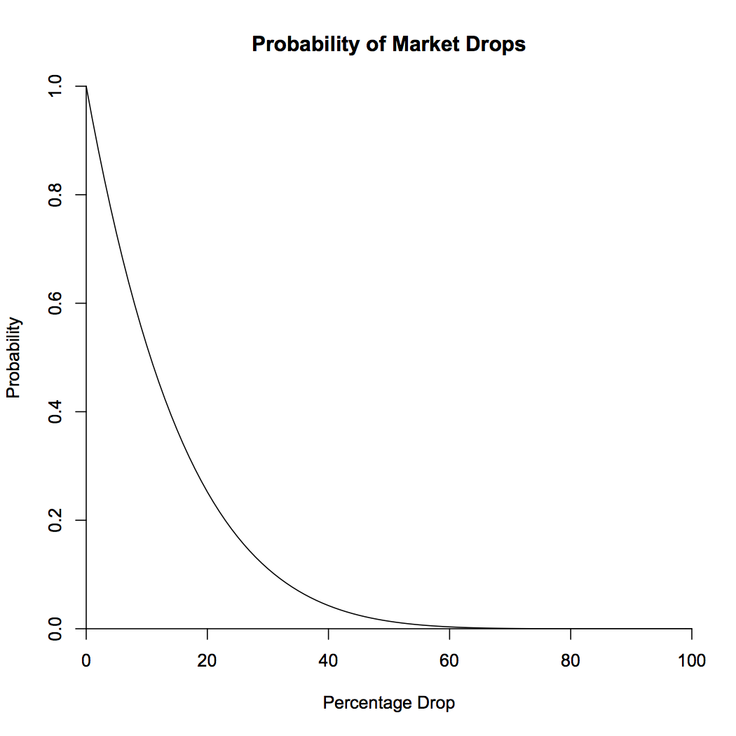
Finally! The hard math is done, and we can reap our rewards. Plugging in \(\mu = .10\), \(\sigma = .18\), and \(a = -.062\), we see that the probability that the market will be 6% lower than it is now at some point in the future is a whopping 68%! The probability of a 10% dip, which corresponds to a drop of \(-.105\), is 52%, still more likely than not. Eschewing my love of logarithms for a moment, below is a plot showing the probability that a given percentage drop will occur.
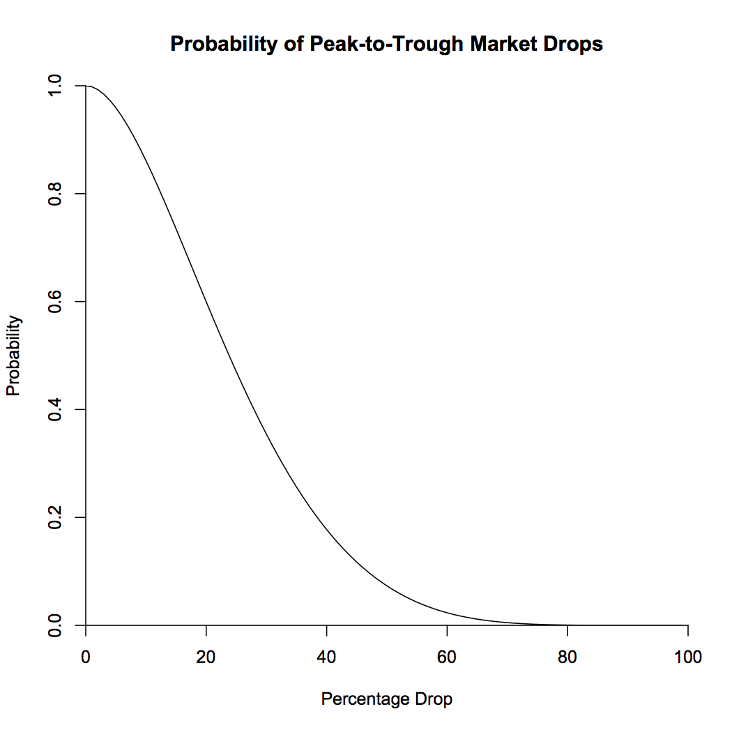
What about the peak-to-trough question that the analysts love? One way to look at it is to notice that if we run the stock market backwards, it’s a Brownian motion with drift \(-\mu\) and the same volatility \(\sigma^2\). We can say that we’re in the midst of a peak-to-trough dip of size at least \(a\) if, looking backwards, we have an increase of \(a_1\), and looking forwards, we have a decrease of \(a_2\), where \(a_1 + a_2 > a\). Now, we notice that \(F(x) = 1 - e^{\frac{-2 \mu x}{\sigma^2}}\) (on the positive reals) is the cumulative density function for the probability distribution of having the biggest future drop be of size \(x\), and by symmetry, of having the biggest gain looking backwards be of size \(x\). So what we want is the probability that \(a_1 + a_2 > a\), where \(a_1\) and \(a_2\) are independent and distributed according to \(F\). This probability is \begin{align*} P(a_1 + a_2 > a) &= \int_{x + y > a} F'(x)F'(y)\,dx\,dy\\ &= \int_{0}^{\infty} F'(x) \int_{\max(a - x, 0)}^{\infty} F'(y)\,dy\,dx\\ &= \frac{2\mu}{\sigma^2} \int_{0}^{a} e^{\frac{-2 \mu a}{\sigma^2}}\,dx + \int_{a}^{\infty} F'(x)\,dx\\ &= e^{\frac{-2 \mu a}{\sigma^2}} \left(1 + \frac{2\mu a}{\sigma^2}\right). \end{align*}
This brings us up to 92% for a 6% drop, and 86% for a 10% drop. What this means is that 92% of the time, the market is in the midst of a peak-to-trough drop of 6%. Note that the way we’ve calculated things does not exclude the possibility of a lower trough between the previous peak and now, or a higher peak between now and the trough. I’ll leave that one as an exercise. The probabilities of percentage drops are shown in the plot below.
So what have we shown here? If we allow ourselves to choose arbitrary endpoints, “correction” is the default state of the market. Half of the time, we can find a peak in the past and a trough in the future that represent a drop of at least 25%! If this seems impossible, let’s check it by looking at actual market data. I looked at monthly returns from 1963 to the present. This range has higher mean returns and lower standard deviation than my typical 10% and 18% (which I use because I like to be a conservative investor), which lowers the probabilities a bit. The plot below shows the probability of peak-to-trough drops from the model with drift and volatility taken from the data, as well as the actual observed frequencies.
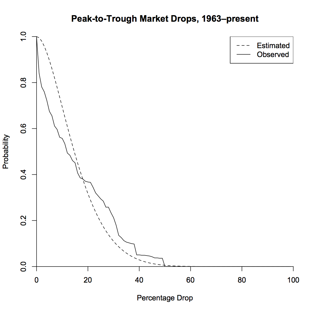
The model greatly overestimates the probabilities of small drops. This is due to the fact that looking at monthly data, rather than instantaneous data, smooths out the peaks and troughs, which will lose a lot of the smaller ones. Also, the market may drop in the future, which would lead to an increase in drops over this timespan. But overall, the model looks like it fits pretty well! Let’s take a look at the time series, colored by the size of the peak-to-trough drop.
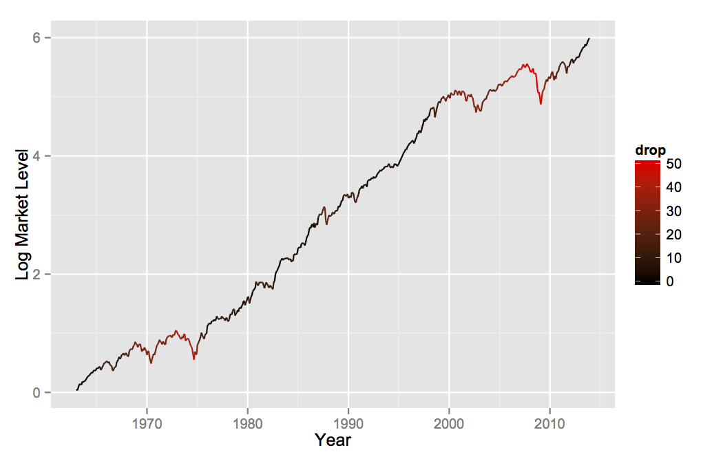
So what we’ve shown is that when you measure corrections from a previous peak to a future trough, we’re almost always in a big correction. Even taking the more honest accounting of only looking at drops going forwards, you can still be pretty sure you’ll be down at least 5% or so from where you are now. You can tell yourself stories about scared investors or emerging market currencies, but ultimately, the existence of corrections is due to the high level of market volatility. The goal of financial analysis should be to explain that volatility directly, rather than to try to pick apart individual market fluctuations ex-post. Financial navel-gazing makes for good television, but it does little to help our understanding of markets.