Telling Stories about Market Corrections
Much of the financial news over the past couple of weeks has centered on the question of whether the stock market is in the midst of a “correction.” The S&P 500 index peaked near 1,850 before taking a plunge which bottomed out near 1,740 (unless, of course, the gains of the last few days reverse themselves once again). A drop from 1,850 to 1,740 represents a 6% decline, which is huge when you consider that the market averages an increase of about 10% per year. So the analysts start trotting out stories about why this happened: the market was overvalued and was “due” to correct, investors got scared by a collapse of emerging market currencies, yadda yadda yadda. It’s easy to make up stories about why something happened in the past because nobody can tell you you’re wrong. I prefer the challenge of telling stories with enduring lessons to learn. Today’s story is about Brownian motion and why we should probably attribute market corrections to dumb luck.
Before I begin the story, I want to spend a moment to talk to you about logarithms. I plan on devoting an entire post, or possibly several entire posts, to logarithms, but for now, let me just assure you that your life will become so much easier once you embrace the logarithm. So instead of thinking about the level of the S&P 500 index, let’s think of the log level. So our 6% (arithmetic) decline represents a change of \(\log(1 - .06) \approx -.062\) in the log level. The nearness of \(x\) and \(\log(1 + x)\) for small values of \(x\) is frustrating, because it makes it seem like there’s no difference between taking log changes and not. There’s a huge difference! If the market drops by 6% every month from now to eternity, we can just keep subtracting \(-.062\) from the log level, but you’ll be burdened with pesky multiplications if you try to remain arithmetic. So when we talk about the stock market from now on, we’ll mean the log level of the market.
One of the simplest and most enduring models of the stock market is as a Brownian motion with drift \(\mu\) and volatility \(\sigma^2\). The past tells us that \(\mu\) is about .10 per year, and \(\sigma^2\) is about \(.18^2\) per year. What this means is that our best guess for the level of the market \(t\) years from today is that it is normally distributed with a mean \(\mu t = .10t\) higher than it is now and a variance of \(\sigma^2 t = (.18)^2 t\). Now, let me make it clear that this model is wrong, not because continuous time and real numbers aren’t real (they aren’t, but that doesn’t really matter here), but because there are variables that can forecast expected returns, so our best guess is actually better than this. Nevertheless, the story of Brownian motion captures much of how we should think about the stock market over short time periods (days, weeks, months).
Now that we have a model, we can ask: how often should we expect a correction of a given magnitude? This is actually a pretty stupid question the way that the talking heads on CNBC think about it, because they’ll measure a correction from peak to trough. But what good is that to an investor, when you can’t know until after the fact that you’ve hit a peak or a trough? So let me start with a more fundamental question: what is the probability that at some point in the future the market will be down \(-.062\) from the price today? (Notice that this implies a larger correction from the peak, because with probability 1 you’ll see a higher market level before the drop! But let’s hold off on that disturbing thought for now.)
The way to approach this problem involves using a supremely valuable tool from the stochastic calculus toolbox: change of measure. Asking this sort of question for a driftless Brownian motion is easy: a driftless Brownian motion will always experience a \(-.062\) correction! So what we’ll do is we’ll just realize our Brownian motion with drift as just an ordinary driftless Brownian motion, but under a different measure.
We will write our market process in differential form as \[dX_t = \mu\,dt + \sigma\,dB^Q_t,\] where \(X_t\) is the (log) market level, and \(B_t\) is a standard Brownian motion with respect to a probability measure \(Q\). What we want is that the measure \(Q\) is equivalent to the standard measure \(P\) such that \(dX_t = \sigma dB^P_t\), where \(B^P_t\) is standard Brownian motion under \(P\). Plugging in \(\sigma dB^P_t\) for \(dX_t\) above gives \[\sigma dB^P_t = \mu\,dt + \sigma\,dB^Q_t,\] or \[dB^P_t = \frac{\mu}{\sigma} \,dt + dB^Q_t.\]
The magic wand we will wave over this is a result called the Girsanov theorem. In a nutshell, it says that if \(A_t\) is a sufficiently nice process, then we can find a change of measure such that \[dB^P_t = A_t\,dt + dB^Q_t.\] Here we have the very special case where \(A_t\) is a constant, \(\frac{\mu}{\sigma}\). Girsanov tells us to construct a process \(M\) such that \[dM_t = A_tM_t\,dB^P_t, \quad M_0 = 1.\] This stochastic differential equation has a simple solution, given by the so-called stochastic exponential: \[M_t = e^{\int_0^t A_s\,dB^P_s - \frac{1}{2}\int_0^t A_s^2\,ds}.\] In our case, \(A_t = \frac{\mu}{\sigma}\), so this becomes \[M_t = e^{\frac{\mu}{\sigma} B^P_t - \frac{\mu^2}{2\sigma^2} t}.\] (Exercise: Use your mad Itō’s lemma skillz to check that this \(M\) satisfies the desired SDE.) With this process in hand, Girsanov tells us that, provided it is a martingale, the measures \(Q\) and \(P\) are related by \[\frac{dQ}{dP} = M_t\] for an arbitrary value of \(t\). (Another exercise: Show, using the assumption that \(M_t\) is a martingale, that the value of \(t\) doesn’t actually matter as long as we’re considering things at time \(s \leq t\). So we just take \(t\) to be as large as we need.)
Whew! Take a deep breath! Let’s remember what we’re trying to do: we want to find the \(Q\)-probability that our market process \(X_t\) dips below some level \(a\) (\(-.062\), for example). We’ve engineered things such that \(X_t = \sigma dB^P_t\). Let’s write \[T_a = \inf \{t \in \mathbb{R} \mid \sigma B^P_t = a\} = \inf \{t \in \mathbb{R} \mid B^P_t = \frac{a}{\sigma}\}.\] So our question is, what’s the \(Q\)-probability that \(T_a\) is finite? Well, let’s use the definition the Radon-Nikodym derivative: it’s \[E^P(M_{T_a} \mathbb{1}_{T_a < \infty}).\] But we were clever! Under the measure \(P\), \(T_a\) is finite with probability 1, so we’re left with \begin{align*} Q(T_a < \infty) &= E^P(M_{T_a})\\ &= E^P\left(e^{\frac{\mu}{\sigma} B^P_{T_a} - \frac{\mu^2}{2\sigma^2} T_a}\right)\\ &= e^{\frac{\mu a}{\sigma^2}} E^P\left(e^{-\frac{\mu^2}{2\sigma^2} T_a} \right). \end{align*} Now, we could calculate the remaining expectation, but instead we’ll be sneaky. Observe that if the drift \(\mu\) has the same sign as \(a\), then the \(Q\)-probability has to be 1: of course the stock market will eventually produce a gain of 6%. So in this case, we must have \[ E^P\left(e^{-\frac{\mu^2}{2\sigma^2} T_a} \right) = e^{-\frac{\mu a}{\sigma^2}}.\] But the expression on the left is indifferent to the sign of \(\mu\)! So in the case we’re interested in, where \(\mu\) and \(a\) have different signs, we must have \[ E^P\left(e^{-\frac{\mu^2}{2\sigma^2} T_a} \right) = e^{\frac{\mu a}{\sigma^2}}.\] Thus, \[Q(T_a < \infty) = e^{\frac{\mu a}{\sigma^2}} \cdot e^{\frac{\mu a}{\sigma^2}} = e^{\frac{2 \mu a}{\sigma^2}}.\]
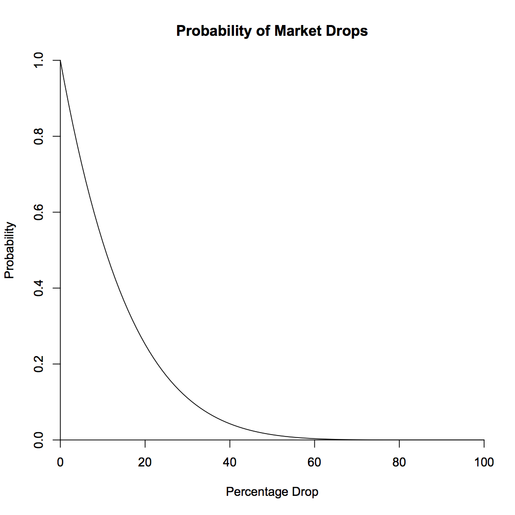
Finally! The hard math is done, and we can reap our rewards. Plugging in \(\mu = .10\), \(\sigma = .18\), and \(a = -.062\), we see that the probability that the market will be 6% lower than it is now at some point in the future is a whopping 68%! The probability of a 10% dip, which corresponds to a drop of \(-.105\), is 52%, still more likely than not. Eschewing my love of logarithms for a moment, below is a plot showing the probability that a given percentage drop will occur.
What about the peak-to-trough question that the analysts love? One way to look at it is to notice that if we run the stock market backwards, it’s a Brownian motion with drift \(-\mu\) and the same volatility \(\sigma^2\). We can say that we’re in the midst of a peak-to-trough dip of size at least \(a\) if, looking backwards, we have an increase of \(a_1\), and looking forwards, we have a decrease of \(a_2\), where \(a_1 + a_2 > a\). Now, we notice that \(F(x) = 1 - e^{\frac{-2 \mu x}{\sigma^2}}\) (on the positive reals) is the cumulative density function for the probability distribution of having the biggest future drop be of size \(x\), and by symmetry, of having the biggest gain looking backwards be of size \(x\). So what we want is the probability that \(a_1 + a_2 > a\), where \(a_1\) and \(a_2\) are independent and distributed according to \(F\). This probability is \begin{align*} P(a_1 + a_2 > a) &= \int_{x + y > a} F'(x)F'(y)\,dx\,dy\\ &= \int_{0}^{\infty} F'(x) \int_{\max(a - x, 0)}^{\infty} F'(y)\,dy\,dx\\ &= \frac{2\mu}{\sigma^2} \int_{0}^{a} e^{\frac{-2 \mu a}{\sigma^2}}\,dx + \int_{a}^{\infty} F'(x)\,dx\\ &= e^{\frac{-2 \mu a}{\sigma^2}} \left(1 + \frac{2\mu a}{\sigma^2}\right). \end{align*}
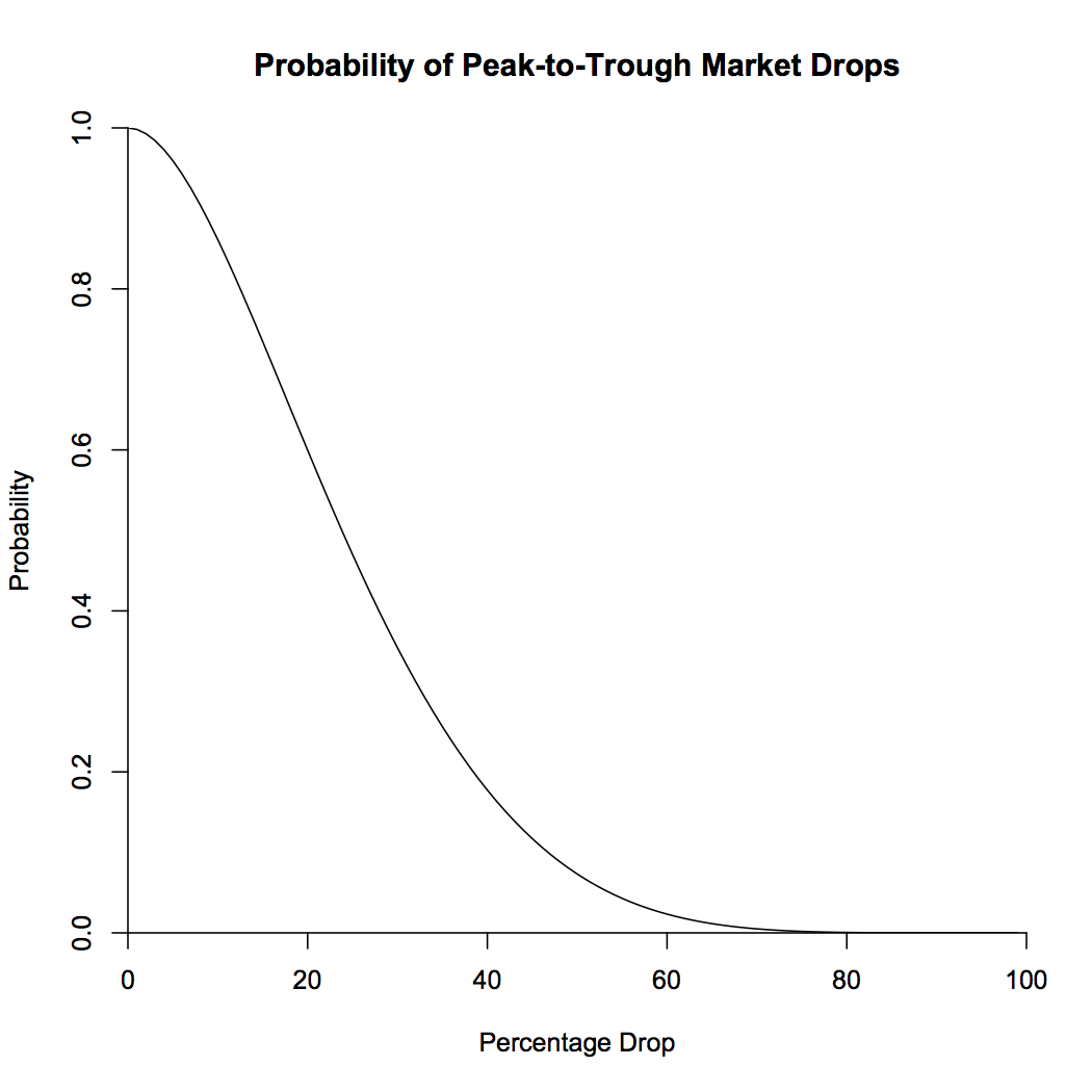
This brings us up to 92% for a 6% drop, and 86% for a 10% drop. What this means is that 92% of the time, the market is in the midst of a peak-to-trough drop of 6%. Note that the way we’ve calculated things does not exclude the possibility of a lower trough between the previous peak and now, or a higher peak between now and the trough. I’ll leave that one as an exercise. The probabilities of percentage drops are shown in the plot below.
So what have we shown here? If we allow ourselves to choose arbitrary endpoints, “correction” is the default state of the market. Half of the time, we can find a peak in the past and a trough in the future that represent a drop of at least 25%! If this seems impossible, let’s check it by looking at actual market data. I looked at monthly returns from 1963 to the present. This range has higher mean returns and lower standard deviation than my typical 10% and 18% (which I use because I like to be a conservative investor), which lowers the probabilities a bit. The plot below shows the probability of peak-to-trough drops from the model with drift and volatility taken from the data, as well as the actual observed frequencies.
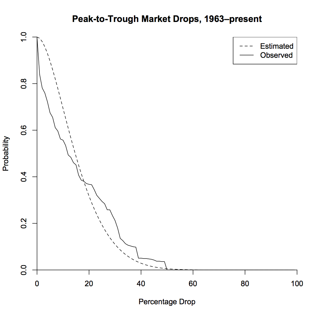
The model greatly overestimates the probabilities of small drops. This is due to the fact that looking at monthly data, rather than instantaneous data, smooths out the peaks and troughs, which will lose a lot of the smaller ones. Also, the market may drop in the future, which would lead to an increase in drops over this timespan. But overall, the model looks like it fits pretty well! Let’s take a look at the time series, colored by the size of the peak-to-trough drop.
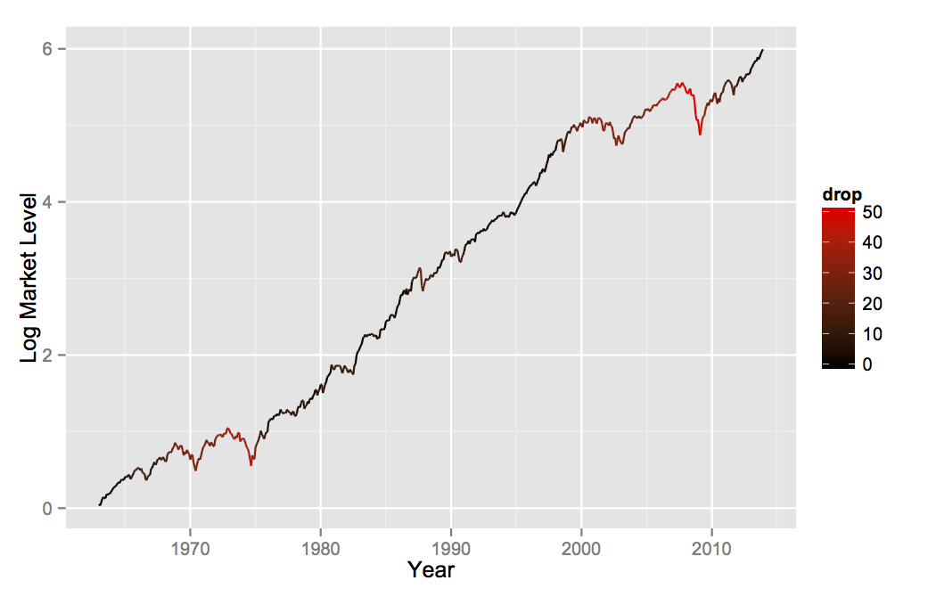
So what we’ve shown is that when you measure corrections from a previous peak to a future trough, we’re almost always in a big correction. Even taking the more honest accounting of only looking at drops going forwards, you can still be pretty sure you’ll be down at least 5% or so from where you are now. You can tell yourself stories about scared investors or emerging market currencies, but ultimately, the existence of corrections is due to the high level of market volatility. The goal of financial analysis should be to explain that volatility directly, rather than to try to pick apart individual market fluctuations ex-post. Financial navel-gazing makes for good television, but it does little to help our understanding of markets.